There is a relationship, Taylor’s Law, that has the potential to reveal crime data manipulation.
This is useful considering Tom Winsor of HMIC told the Home Affairs Select Committee last year, that the questions of whether officers are fiddling data is “where, how much (and) how severe”.
Before exploring these issues, I should explain that my interest in this project started with a request for a department seminar. My name is Quentin Hanley, I work in a combined Chemistry and Forensics Department at Nottingham Trent University and I was looking for ways to make statistical concepts more relevant to Forensic Science students who might attend my seminar. This culminated in a paper I co-authored – Fluctuation Scaling, Taylor’s Law and Crime which is free to view online.
But first of all, a few explanations are needed to help you better understand how something called Taylor’s Law can reveal characteristics of the recording process leading to the crime report statistics.
What is Taylor’s law?
Taylor’s power law is named after an academic ecologist named Roy (L. R.) Taylor who in 1961 observed a simple mathematical relationship between the density of a species population and how much it varied in a given area. Taylor saw the same relationship in 24 different species ranging from beetles to fish. Taylor’s simple method has made it possible to estimate much more precisely what a given future population size could look like and how it might fluctuate. Taylor’s law has been applied far and wide within ecology to determine the potential for species extinction or the transmission of infectious diseases. By way of example, this paper shows how very small and isolated reefs had much higher than expected temporal variance in fish abundance. From its beginnings in ecology, Taylor’s law has since been applied to currency trading, urban traffic, and human disease. Applying Taylor’s Law begins with a mean variance plot.
What is mean variance?
Mean variance is a mathematical way of estimating how much variation you can expect around an average. One version is often used in finance where the variance represents the range of volatility in the prices of given assets and the mean is the averaged plot line that runs through this range and determines the expected financial return. The mean variance approach can also be used to measure the gain of an amplifier.
What is gain?
Gain is a measure of how two (or more) systems respond to the same input. For example, recordings of noise from airplanes, traffic, or a party can be loud or quiet depending on the gain setting of the volume control on the amplifier playing them back to us. However, the volume does not influence our ability to identify what we are hearing. Traffic does not sound like a party and our ears can discern the unique signatures. With the assistance of Taylor’s law we can begin to discern the unique signatures of different types of crime AND measure the relative gain of their recording.
How does gain apply to crime?
In the case of crime, the noise is not from an airplane or party, it is the fluctuations in crime over time. These fluctuations are recorded by a police force and played back to us in the form of police crime report statistics. If we know something about the statistical distribution describing a type of crime, we can measure the relative gain of a particular police force and ask if some Constabularies are “loud” and others “quiet.”
What is a statistical distribution?
Most people are aware of the bell shaped curve of the “normal” distribution first proposed by Gauss in 1809. The normal distribution, unfortunately, does not apply to countable things or events like crime reports. For that we need something like the Poisson distribution named after Simeon Denis Poisson who first described it in 1837.
What is special about the Poisson Distribution?
The Poisson distribution applies to many countable things such as photons of light, accidents, and, in the absence of “clumping,” yeast cells in beer. It also gives a reference point in a Taylor’s Law analysis corresponding to things that are not being clustered together and appear random. Against this reference point we can observe that some events are nearly random such as reports of violence in Nottinghamshire and Derbyshire and others events show greater clustering like burglary in those same regions. Beginning with the Poisson distribution as a reference point we can start to evaluate manipulation.
What is manipulation?
Police officers have been the focus of testimony before parliament related to manipulation of statistics. However, in this context I take manipulation to be anything that alters the process of recording crime statistics resulting in an imperfect representation of the original events. Manipulation can be many things and the conscious behaviour of individual officers is only one.
How might manipulation work?
Consider a Constable confronted with a group of five youths playing in a municipal fountain shouting insults and splashing water on passers-by. Many outcomes are possible. After an intervention, it is possible that no further action is taken. Alternatively, the Constable might decide this was anti-social behaviour and file a report. It might also be possible the Officer is called to a more serious problem leaving this incident with no action taken at all.
The eventual outcome could be influenced by staffing in the constabulary. If staffing is low the probability of moving on to more serious matters will increase.
The outcome could also be influenced by policing targets or quotas. For example, if Constables are subject to an anti-social behaviour reporting target, this incident might represent an opportunity to reach that target increasing the incentive to file a report. If the target for a particular reporting period has been met, there might be less incentive to file a report. Depending on training, policies, and incentives, this could represent as many as five reports (one for each youth) resulting in a “loud” response or only one giving a “quieter” response.
The outcome might be influenced by a threshold effect with the first few incidents drawing no police attention, but after more occur this might change.
When looked at this way, it is less obvious how this should be recorded, particularly in a Force with limited resources. This scenario may be simplistic but this Wall Street Journal article on possible stop-and-frisk and arrest quotas in the New York Police Department may provide perspective. The important point is that Taylor’s law plots can help find and assess some of these manipulative influences.
How does this all fit together?
In approaching this research, the idea was to show an example of the method of mean-variance I had used many years ago to characterise the gain of digital camera sensors similar to those used in phones. The method uses the statistical properties of light (Poisson distribution) to measure the gain of a detector.
Since crime reports, light photons, are countable, I wondered if they would behave like photons and have similar predictable mean variance behaviour.
I started looking at crime statistics from a few neighbourhoods. An individual neighbourhood might look like the figure below which shows how crime fluctuates (whatever the short term trends might be).
Realising the growing scope of this work after looking at a only a few neighbourhoods, I knew I needed assistance. Fortunately, last year, 3 exceptional students (my co-authors Amal, Rachel, and Suniya) volunteered to work for me. They did some chemistry during their time, but were also willing to help with this study. We divided up the work and started assembling a data set.
You will now understand that crime reports are signals produced by a detection system (the police) reporting on crimes committed. If everything turned out as I expected, a plot with the average number of crime reports per month on the x-axis and variance on the y-axis would have a slope of one (linear scaling law). If all Constabularies have the same amplification, the gain would also be the same for all of them.
The data did not show the anticipated results (do they ever?). Crime reports from policing neighbourhoods followed the more complex scaling relationship represented by Taylor’s Law. It certainly did not look like a Poisson distribution.
By the time of my departmental seminar (December 2013) the results looked like this:
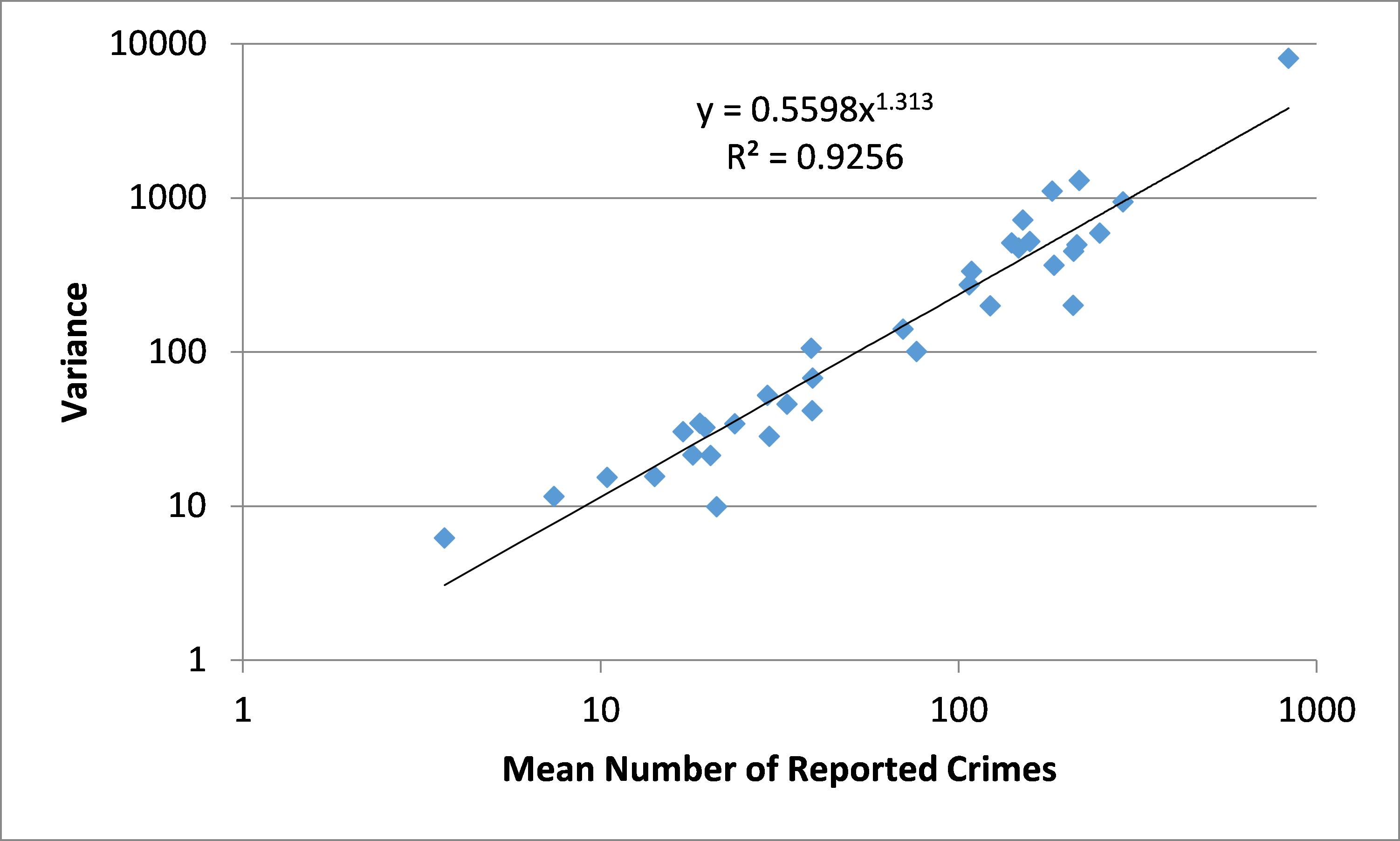
Where we expected a straight line with a slope of one, we observed a power law with an exponent of 1.313 and where the slope should have been was a factor of 0.5598 (not 1!). This data was a mix of violence (lower values) and total crime (larger values) as we did not know at the time that mixing crime types was not a good practice.
Convinced that a relationship could be discovered, we systematically looked at all 151 policing neighbourhoods in Nottinghamshire and Derbyshire. We looked at different types of crime as categorised in the Police statistics. We also looked at larger scale data sets from UKCrimeStats and at less controversial statistics (mortality) for comparison. The results have now been published and there are three particularly useful conclusions:
- The relative gain of a Constabulary can be measured by using data from their policing neighbourhoods and comparing it to another Constabulary. Using Derbyshire as the reference, Nottinghamshire showed a “louder” gain (1.36) for anti-social behaviour, and a “quieter” response (0.73) for burglary. In these two regions, violence and total crime had identical gain within statistical limits. These measurements provide a more rigorous and defensible way to compare Forces than unadjusted crime reports.
- Some types of crime show greater clustering. Violence in policing neighbourhoods appears randomly distributed while “other crime”, which includes many crimes of deceit, is more highly clustered.
- Police statistics have been criticised due to widely reported manipulation. Using simple models, we found that some types of manipulation are obvious in a mean-variance plot.
Crime reports from neighborhoods follow a Law, Taylor’s Law. Using this as a starting point, we can extract useful information such as relative gain from imperfect crime statistics provided by the Police. Overall when compared to transmission of measles, total crime at local scale clusters similarly to measles in a population in which 80-90% of people are vaccinated.
I have savoured researching this paper. I’m of the view there is still much more analysis that can be done using sophisticated statistical analysis of available crime data. I now look forward to taking this work further, across all UK Police Forces and attempt to look at other countries. I’d be happy to answer any queries and you can contact me at Quentin.hanley[AT]ntu.ac.uk .